Are you sure you want to delete this task? Once this task is deleted, it cannot be recovered.
You can not select more than 25 topics
Topics must start with a chinese character,a letter or number, can include dashes ('-') and can be up to 35 characters long.
 yehua
0a1c137f37
yehua
0a1c137f37
|
1 year ago | |
|---|---|---|
| pytorch | 1 year ago | |
| BDresult.png | 2 years ago | |
| Improved Deep Point Cloud Geometry Compression.pdf | 2 years ago | |
| LICENSE | 1 year ago | |
| OpenPointCloud-logo.png | 1 year ago | |
| README - old-2.md | 1 year ago | |
| README - old.md | 1 year ago | |
| README.md | 1 year ago | |
| compression-1.3.zip | 2 years ago | |
| flowchart.vsdx | 2 years ago | |
| pc_error_d | 2 years ago | |
| pcc_geo_cnn_v2_D1.png | 2 years ago | |
| pcc_geo_cnn_v2_D2.png | 2 years ago | |
| requirements-pytorch.txt | 1 year ago | |
| result-final.xlsx | 1 year ago | |
| test_result.xlsx | 2 years ago | |
| tmc3 | 2 years ago | |
README.md
![]()
pcc_geo_cnn_v2
point clouds, compression, neural networks, geometry, octree
pcc_geo_cnn_v2 is based on pcc_geo_cnn_v1, for lossy point cloud compression. And for performance optimization, the author comes up with 5 thoughts, and verifies them by experiments.
our contributions
1.benchmark test on different PC files, and on different metrics, including bpp, D1, D2, time, compared TensorFlow with pytorch.
2.draw a flow chart about encoding process.
3.BD-BR and BD-PSNR calculation over GPCC(octree), also compared with pcc_geo_cnn_v1.
4.transplant from tensorflow to pytorch
file structure
root
└── TensorFlow code
└── compression-1.3.zip: TensorFlow-compression module
└── pytorch: pytorch version code, models included
└── Improved Deep Point Cloud Geometry Compression.pdf: origional paper
└── flowchart.vsdx: flow chart about encoding process
└── trainsets: ModelNet40_200_pc512_oct3_4k.zip converted from ModelNet40
└── pc_error_d: gpcc metrics software
└── tmc3: gpcc compression software
environment
- pytorch
- ubuntu 18.04
- cuda V10.2.89
- python 3.6.9
- refer to requirements-pytorch.txt
command
- pytorch
cd pytorch
Training:
python train_new.py
Compress/Decompress:
python compress_octree.py --input_files "/userhome/PCGCv1/pytorch_eval/28_airplane_0270.ply" --output_files '28_airplane_0270.ply.bin' --input_normals "/userhome/PCGCv1/pytorch_eval/28_airplane_0270.ply" --dec_files '28_airplane_0270.ply.bin.ply' --checkpoint_dir 'models/5.0e-5/epoch_96.pth'
performance
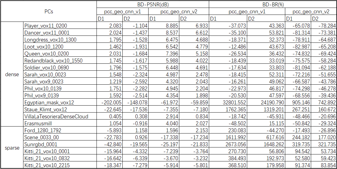
We first caculate the BD-PSNR and BD-BR rate of pcc_geo_cnn_v2 with the model of c4-ws, which has the best performance than others, over GPCC(octree), the result shows as below. We can see from the table, that for dense PC with bitwidth of 10 and 11, pcc_geo_cnn_v2 gets better performance over octree, while for sparse or vox12 PC, it gets worse. The main reason is that there is no PC data in training sets with similar distributions or geometry features. Compared with pcc_geo_cnn_v1, pcc_geo_cnn_v2 has better performance, no matter for dense or sparse, or other bitwidth.
We then carry out a benchmark test on PC files both on TensorFlow and Pytorch, including those are not tested by author. The result shows below. From the result, we can see that the bpp of pytorch is much smaller than tensorflow, while d1 and d2 is just a little bit smaller, it may be because we adjust the lmbda parameter to get best performance for pytorch. As for running time, pytorch takes less time, for the faster speed of 3d convolution operation.
| PC files | TF_bpp | TF_d1 | TF_d2 | TF_Enc_Dec_time | PT_bpp | PT_d1 | PT_d2 | PT_Enc_dec_time |
|---|---|---|---|---|---|---|---|---|
| queen_vox10_0200.ply | 0.692 | 75.759 | 79.388 | 1469.03 | 0.385 | 74.798 | 77.93 | 1364.85 |
| longdress_vox10_1300.ply | 0.885 | 74.75 | 78.481 | 1896.43 | 0.483 | 73.518 | 76.717 | 1369.51 |
| basketball_player_vox11_00000200.ply | 0.872 | 82.321 | 86.291 | 3133.21 | 0.464 | 80.7 | 83.963 | 4989.24 |
| loot_vox10_1200.ply | 0.887 | 75.119 | 78.854 | 1683.22 | 0.482 | 73.859 | 77.037 | 1383.46 |
| dancer_vox11_00000001.ply | 0.848 | 82.376 | 86.314 | 2686.44 | 0.455 | 80.733 | 83.86 | 4377.09 |
| soldier_vox10_0690.ply | 0.915 | 74.908 | 78.689 | 2480.98 | 0.498 | 73.563 | 76.781 | 1740.23 |
| sarah_vox9_0023.ply | 0.891 | 66.564 | 70.048 | 1835.59 | 0.474 | 65.759 | 68.818 | 424.65 |
| sarah_vox10_0023.ply | 0.79 | 72.492 | 75.916 | 2548.6 | 0.434 | 71.838 | 74.84 | 1642.06 |
| phil_vox9_0139.ply | 0.892 | 66.164 | 69.615 | 1928.87 | 0.473 | 65.957 | 69.14 | 394.04 |
| phil_vox10_0139.ply | 0.807 | 72.197 | 75.622 | 2549.86 | 0.44 | 71.476 | 74.564 | 1727.18 |
| redandblack_vox10_1550.ply | 0.91 | 74.082 | 77.674 | 1390.07 | 0.496 | 72.904 | 76.05 | 951.54 |
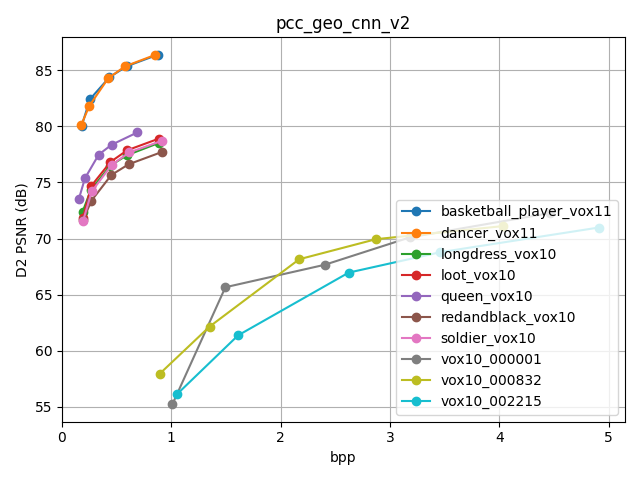
We also draw D1-bpp and D2-bpp figures, to clearly show the performance between different PC files as below. It is obvious that, PCs of vox11 have best performance, which are on up-left part of the figure, PCs of vox10 are second in the middle, and PCs of sparse have bad performance on the bottom part.

Cite from:
@misc{quach2020improved,
    title={Improved Deep Point Cloud Geometry Compression},
    author={Maurice Quach and Giuseppe Valenzise and Frederic Dufaux},
    year={2020},
    eprint={2006.09043},
    archivePrefix={arXiv},
    primaryClass={cs.CV}
}
contributors
name: Ye Hua
email: yeh@pcl.ac.cn
point clouds, compression, neural networks, geometry, octree
Text Python Markdown other
MIT
