PCGCv1_yehua
PCGCv1, point cloud compression, deeplearning, hyper
PCGCv1 is a kind of lossy point cloud compression method. It uses hyper priors to improve performance. The source code uses Tensorflow as deeplearning framework, here we transplant to tensorlayer and pytorch.
Paper Citation:
@ARTICLE{9321375, author={Wang, Jianqiang and Zhu, Hao and Liu, Haojie and Ma, Zhan}, journal={IEEE Transactions on Circuits and Systems for Video Technology}, title={Lossy Point Cloud Geometry Compression via End-to-End Learning}, year={2021}, volume={31}, number={12}, pages={4909-4923}, doi={10.1109/TCSVT.2021.3051377}}
our contributions
1.transplant from TensorFlow to tensorlayer and pytorch.
2.benchmark tests on many PCs, including those not tested by author.
3.BD-BR and BD-PSNR calculation over GPCC(octree), also compared to trisoup.
4.draw a flow chart about encoding process to help better understanding.
files
1.trainingset:refer to points64_part1.zip
2.testset:refer to testdata.zip
3.PCGCv1-master:source code and models on tensorflow
4.pytorch:code and model file on pytorch
5.author results:test results on TF by author
6.tensorlayer:code and model file on tensorlayer
7.Lossy Point Cloud Geometry Compression via End-to-End Learning.pdf:origional paper
8.PCGCv1 performance.xlsx:performance test result between different frameworks
9.PCGCv1 explanation.docx:introduction for paper, migration, instructions
10.flowchart.vsdx:flow chart about encoding process
11.results: test results by contributors
environment
refer to PCGCv1-master/README.md and 'PCGCv1 explanation.docx'
command
1.pytorch
training:
python train.py
encode:
python test.py compress --input=".../redandblack_vox10_1550.ply" --ckpt_dir=".../epoch_13_12599.pth" --batch_parallel=64
decode:
python test.py decompress --input="compressed/longdress_vox10_1300" --ckpt_dir=".../epoch_13_12599.pth"
evaluate:
python eval.py --input ".../longdress_vox10_1300.ply" --ckpt_dir=".../epoch_13_12599.pth"
2.tensorlayer
training:
python train.py
encode:
python test.py compress --input=".../redandblack_vox10_1550.ply" --ckpt_dir=".../ epoch_18_18199.npz" --batch_parallel=4
decode:
python test.py decompress --input="compressed/longdress_vox10_1300" --ckpt_dir=".../ epoch_18_18199.npz"
evaluate:
python eval.py --input ".../longdress_vox10_1300.ply" --ckpt_dir=".../ epoch_18_18199.npz "
performance
We first caculate the BD-PSNR and BD-BR rate of PCGCv1 and GPCC trisoup over GPCC octree on many PCs, the result shows as below. We can see from the table, that for dense PC with bit width of 10 and 11, PCGCv1 gets better performance over octree and trisoup, while for sparse or vox12 PC, it gets worse. The main reason is that there is no PC data in training sets with similar distributions or geometry features.
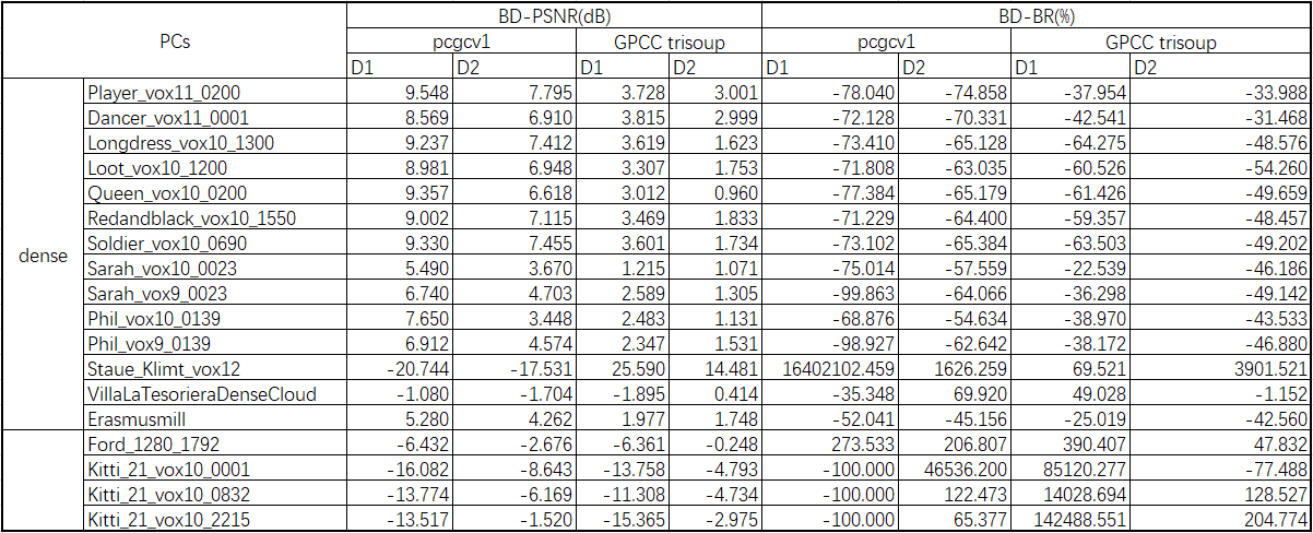
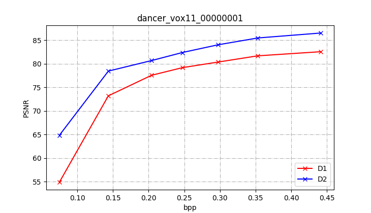
We then carry out a benchmark test on PC files including those are not tested by author. The part of the result shows below. For other results, please go to results/
| PC |
ori_points |
mseF,PSNR (p2plane) |
mseF,PSNR (p2point) |
time_enc |
time_dec |
bpp |
| dancer_vox11_00000001 |
2592758 |
64.8441 |
54.8887 |
227.178 |
102.736 |
0.0749 |
| dancer_vox11_00000001 |
2592758 |
78.4461 |
73.2022 |
191.143 |
90.484 |
0.1435 |
| dancer_vox11_00000001 |
2592758 |
80.6868 |
77.5656 |
205.569 |
83.532 |
0.2042 |
| dancer_vox11_00000001 |
2592758 |
82.3931 |
79.1803 |
222.561 |
88.975 |
0.2474 |
| dancer_vox11_00000001 |
2592758 |
84.0262 |
80.365 |
217.477 |
91.633 |
0.2973 |
| dancer_vox11_00000001 |
2592758 |
85.4772 |
81.6887 |
215.09 |
89.23 |
0.3531 |
| dancer_vox11_00000001 |
2592758 |
86.5282 |
82.5652 |
215.356 |
107.351 |
0.4415 |
| PC |
ori_points |
mseF,PSNR (p2plane) |
mseF,PSNR (p2point) |
time_enc |
time_dec |
bpp |
| sarah_vox9_0023 |
299363 |
57.7055 |
50.695 |
33.071 |
17.38 |
0.0889 |
| sarah_vox9_0023 |
299363 |
64.4054 |
61.5184 |
26.308 |
12.194 |
0.1417 |
| sarah_vox9_0023 |
299363 |
67.2605 |
63.8802 |
27.383 |
12.014 |
0.2254 |
| sarah_vox9_0023 |
299363 |
68.5138 |
65.0884 |
36.251 |
16.083 |
0.2746 |
| sarah_vox9_0023 |
299363 |
69.2561 |
65.7159 |
34.676 |
12.428 |
0.3361 |
| sarah_vox9_0023 |
299363 |
69.9792 |
66.3444 |
32.836 |
12.619 |
0.4053 |
| sarah_vox9_0023 |
299363 |
70.3887 |
66.4396 |
32.061 |
15.015 |
0.5022 |
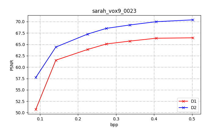
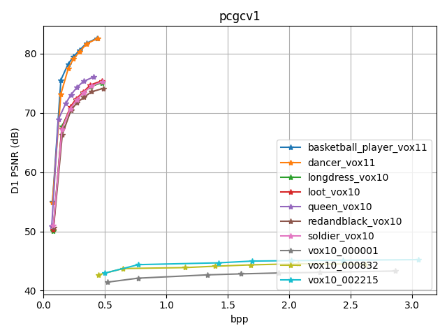
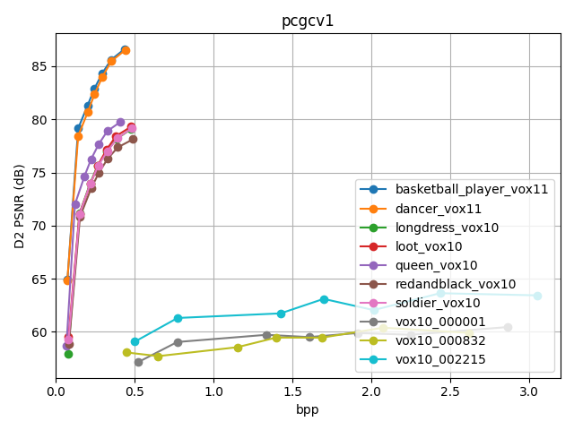
According to the results above, we draw D1-bpp and D2-bpp figures, to clearly show the performance between different PC files as below. It is obvious that, PCs of vox11 have best performance, which are on up-left part of the figure, PCs of vox10 are second in the middle, and PCs of sparse have bad performance on the bottom part.
Cite from:
https://github.com/NJUVISION/PCGCv1
The source code files are provided by Nanjing University Vision Lab. And thanks for the help from SJTU Cooperative Medianet Innovation Center. Please contact us (wangjq@smail.nju.edu.cn) if you have any questions.
contributors
name: Ye Hua
email: yeh@pcl.ac.cn